Study:
Traders often look for “oversold” stocks to get long. Our trading group recently discussed if using common technical analysis metrics like RSI (Relative Strength Index), could be used to find these opportune entries using options?
- Calculate the historical closing 14 day RSI
- Identify when the previous day close was below 30 RSI (oversold) and then crossed above
- Open a short put closest to 30 delta and 45 DTE and hold to expiration
- Analyze the results and compare to random entry groups
- calculate the number of trades entered in the period Jan 2012 - Mar 2018
- sample that same number of trades 1000 times
- compare results of these buckets against RSI entry criteria trades
Results:
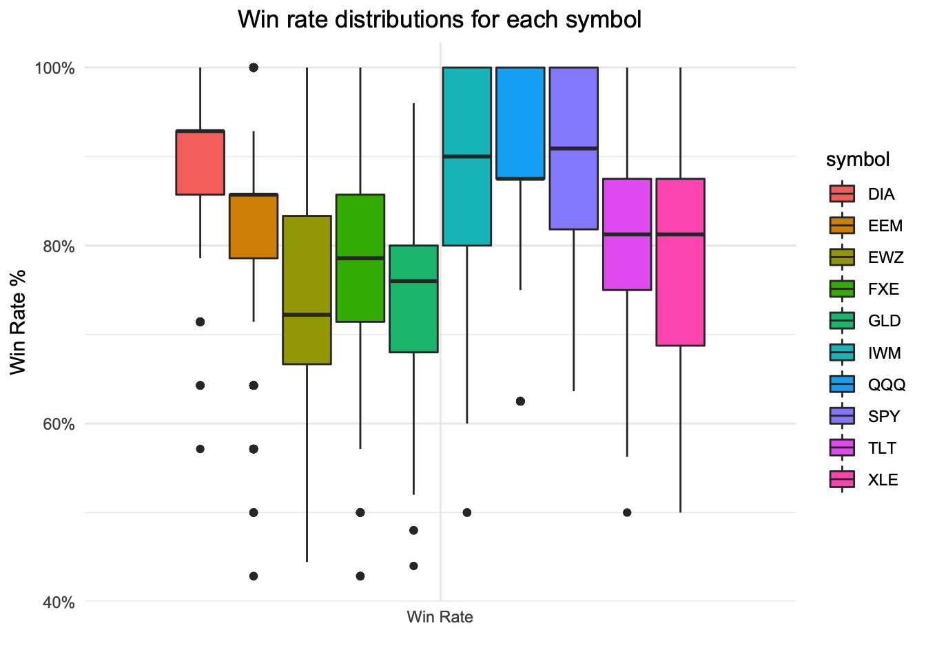
The broad market (ETFs SPY, IWM, QQQ, and DIA) do seem to show a statistically significant improvement in performance over randomly selecting trades over the same time period. Win percentages, Mean profits, and Total profits all ranking in the upper quartiles of random sampling.
FXE in contrast resulted in one of the worst groups of trades in the samples taken.
A few ideas on how to extend this study further:
- Modify from short puts to short put verticals (possibly remove large losses)
- Implement exits at 50% profit rather than expiration only
Setup global options, load libraries:
knitr::opts_chunk$set(message = FALSE, tidy.opts = list(width.cutoff = 60))
suppressWarnings(suppressMessages(suppressPackageStartupMessages({
  library_list <- c("tidyverse", "tastytrade", "here", "TTR",
                    "formattable", "kableExtra", "knitr", "scales")
  lapply(library_list, require, character.only = TRUE)})))
args <- expand.grid(symbol = c("SPY", "IWM", "GLD", "QQQ", "DIA",
                               "TLT", "XLE", "EEM", "EWZ", "FXE"),
                    tar_dte = 45,
                    tar_delta_put = -0.30,
                    stringsAsFactors = FALSE)
Summary of study function:
- Connect to the dataset in redshift
- Open short puts every day given the target DTE and Delta
- Calculate the 14 day RSI and 1 day lag to determine RSI cross days
- Collect a subset of options data that are possible expiration exits
- Close all trades at expiration and join together results
study <- function(stock, tar_dte, tar_delta_put) {
  rs_conn <- tastytrade::redshift_connect("TASTYTRADE")
  options <- rs_conn %>%
    tbl(stock) %>%
    mutate(m_dte = abs(dte - tar_dte))

  rsi <- options %>%
    distinct(symbol, quotedate, close_price) %>%
    collect() %>%
    mutate(rsi = RSI(close_price, n = 14),
           rsi_lag = lag(rsi, 1),
           quotedate = as.Date(quotedate, format = "%Y-%m-%d"))

  opened_puts <- tastytrade::open_short(options, tar_delta_put, "put")

  sub_options <- options %>%
    filter(quotedate == expiration,
           strike %in% opened_puts$put_strike) %>%
    collect() %>%
    mutate(quotedate = as.Date(quotedate, format = "%Y-%m-%d"),
           expiration = as.Date(expiration, format = "%Y-%m-%d"))

  pmap_dfr(list(list(sub_options), opened_puts$quotedate,
                opened_puts$expiration, list("put"),
                opened_puts$put_strike,
                opened_puts$put_open_credit,
                opened_puts$delta_strike,
                opened_puts$close_price),
           tastytrade::close_short_exp) %>%
    left_join(rsi, by = c("symbol", "open_date" = "quotedate",
                          "open_stock_price" = "close_price"))
}
Run Study
results <- pmap_dfr(list(args$symbol, args$tar_dte, args$tar_delta_put), study)
Resample 1000 times
- Count # of trades for each symbol
- Create arguments list including (symbol, count, 1:1000)
- SPY had 11 days when the RSI crossed above 30
- create 1000 random groups with 11 trades in them
set.seed(42)
grp_args <- results %>%
  group_by(symbol) %>%
  filter(rsi > 30, rsi_lag < 30) %>%
  summarise(count = n()) %>%
  ungroup() %>%
  slice(rep(row_number(), 1000)) %>%
  group_by(symbol) %>%
  mutate(run = row_number()) %>%
  ungroup()

result_sample <- function(df, s, n, x) {
  df %>%
    filter(symbol == s,
           complete.cases(.)) %>%
    sample_n(size = n) %>%
    mutate(run = x)
}

resampled <- pmap_dfr(list(list(results), grp_args$symbol, grp_args$count,
                           grp_args$run), result_sample)
Calculate metrics for all runs so we can see the distribution of random entry selections
- Trade Count
- Win Rate
- Mean Credit
- Mean Profit
- Total Profit
metrics <- resampled %>%
  group_by(symbol, run) %>%
  mutate(trade_count = n(),
         profitable = ifelse(put_profit > 0, 1, 0),
         win_rate = sum(profitable) / trade_count,
         mean_credit = mean(put_credit * 100),
         mean_profit = mean(put_profit * 100),
         total_profit = sum(put_profit * 100)) %>%
  distinct(symbol, trade_count, win_rate, mean_credit,
           mean_profit, total_profit) %>%
  ungroup() %>%
  arrange(desc(win_rate))
Boxplot of Win Rates for random samples
metrics %>%
  select(symbol, win_rate) %>%
  gather(., metric, value, -symbol) %>%
  ggplot(., aes(metric, value, fill = symbol)) +
  geom_boxplot() +
  theme_minimal() +
  theme(plot.title = element_text(hjust = 0.5)) +
  scale_x_discrete(labels = "Win Rate") +
  scale_y_continuous(labels = scales::percent) +
  xlab("") +
  ylab("Win Rate %") +
  ggtitle("Win rate distributions for each symbol")

We see a win rate percentage that exceeds the expected target of ~70% based on the 30 delta entry on average
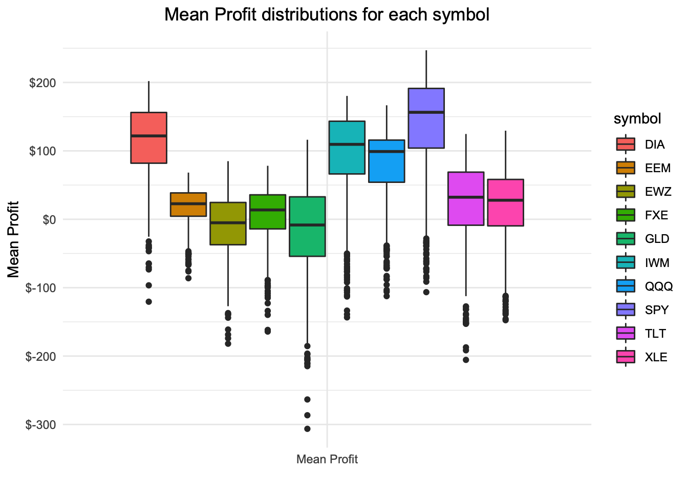
Boxplot of Mean Profit at expiration for random samples
metrics %>%
  select(symbol, mean_profit) %>%
  gather(., metric, value, -symbol) %>%
  ggplot(., aes(metric, value, fill = symbol)) +
  geom_boxplot() +
  theme_minimal() +
  theme(plot.title = element_text(hjust = 0.5)) +
  scale_x_discrete(labels = "Mean Profit") +
  scale_y_continuous(labels = scales::dollar) +
  xlab("") +
  ylab("Mean Profit") +
  ggtitle("Mean Profit distributions for each symbol")

EEM, EWZ, FXE, GLD, TLT, and XLE have distributions of profits at expiration that are not much greater than $0 and may not be showing a strong case for trading the 30 delta short put without additional entry criteria
DIA, IWM, QQQ, and SPY seem to have a more positive distribution of mean profit with random entries
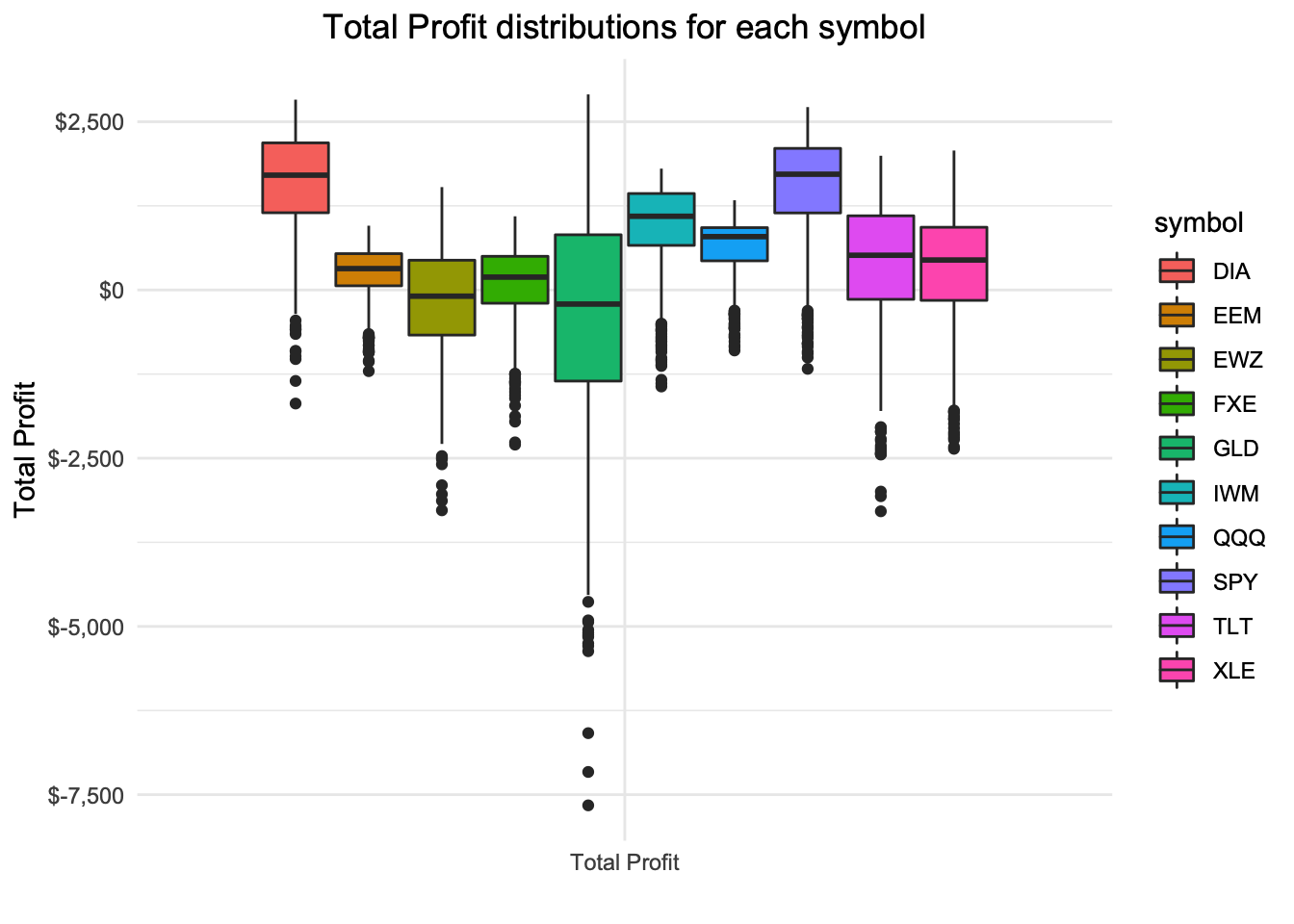
Boxplot of Total Profit at expiration for random samples
metrics %>%
  select(symbol, total_profit) %>%
  gather(., metric, value, -symbol) %>%
  ggplot(., aes(metric, value, fill = symbol)) +
  geom_boxplot() +
  theme_minimal() +
  theme(plot.title = element_text(hjust = 0.5)) +
  scale_x_discrete(labels = "Total Profit") +
  scale_y_continuous(labels = scales::dollar) +
  xlab("") +
  ylab("Total Profit") +
  ggtitle("Total Profit distributions for each symbol")

As expected by the mean profit plot the total profit distributions share the same general outcomes. This gives further evidence that additional criteria my be advantageous or required for this strategy.
Calculate metrics for RSI cross-over entries
- Trade Count
- Win Rate
- Mean Credit
- Mean Profit
- Total Profit
rsi_results <- results %>%
  group_by(symbol) %>%
  filter(rsi > 30, rsi_lag < 30) %>%
  ungroup()

rsi_metrics <- rsi_results %>%
  group_by(symbol) %>%
  mutate(trade_count = n(),
         profitable = ifelse(put_profit > 0, 1, 0),
         win_rate = sum(profitable) / trade_count,
         mean_credit = dollar(mean(put_credit * 100)),
         mean_profit = mean(put_profit * 100),
         mean_profit = ifelse(mean_profit < 0,
                              cell_spec(dollar(mean_profit),
                                        color = "red", italic = TRUE),
                              dollar(mean_profit)),
         total_profit = sum(put_profit * 100),
         total_profit = ifelse(total_profit < 0,
                               cell_spec(dollar(total_profit),
                                         color = "red", italic = TRUE),
                               dollar(total_profit))) %>%
  distinct(symbol, trade_count, win_rate, mean_credit,
           mean_profit, total_profit) %>%
  ungroup() %>%
  arrange(desc(win_rate)) %>%
  mutate(win_rate = percent(win_rate))
Metrics table for RSI cross-over entries
kable(rsi_metrics, digits = 2, format = "html",
      caption = "Metrics for selling puts after cross above RSI 30",
      col.names = c("SYM", "TRADE COUNT", "WIN RATE", "MEAN CREDIT",
                    "MEAN PROFIT", "TOTAL PROFIT"),
      escape = FALSE,
      align = c("l", "r", "r", "r", "r", "r")) %>%
  kable_styling(bootstrap_options = "striped",
                full_width = FALSE) %>%
  column_spec(., 1:6, width = "1.0in")
| SYM | TRADE COUNT | WIN RATE | MEAN CREDIT | MEAN PROFIT | TOTAL PROFIT |
|---|---|---|---|---|---|
| SPY | 11 | 100.0% | $307.68 | $306.64 | $3,373 |
| IWM | 10 | 100.0% | $208.60 | $208.05 | $2,080.50 |
| QQQ | 8 | 100.0% | $155.63 | $155.13 | $1,241 |
| DIA | 14 | 92.9% | $219.61 | $183.89 | $2,574.50 |
| TLT | 16 | 81.2% | $128.44 | $82.31 | $1,317 |
| XLE | 16 | 81.2% | $132.44 | $63.53 | $1,016.50 |
| GLD | 25 | 80.0% | $149.18 | $-3.52 | $-88 |
| EEM | 14 | 78.6% | $73.61 | $10.11 | $141.50 |
| EWZ | 18 | 66.7% | $100.22 | $-59.86 | $-1,077.50 |
| FXE | 14 | 50.0% | $82.86 | $-55.07 | $-771 |
The table above shows that using the RSI cross-over entry leads to at a high level similar results in that the same symbols (DIA, IWM, QQQ, and SPY) perform better overall than the others. Next we will compare these results more closely to see if there is evidence that the RSI indicator enhances the results.
Does RSI cross-over improve results?
compare <- rsi_results %>%
  mutate(run = 1001) %>%
  bind_rows(resampled) %>%
  group_by(symbol, run) %>%
  mutate(trade_count = n(),
         profitable = ifelse(put_profit > 0, 1, 0),
         win_rate = sum(profitable) / trade_count,
         mean_credit = mean(put_credit * 100),
         mean_profit = mean(put_profit * 100),
         total_profit = sum(put_profit * 100)) %>%
  distinct(symbol, trade_count, win_rate, mean_credit,
           mean_profit, total_profit) %>%
  ungroup() %>%
  group_by(symbol) %>%
  arrange(desc(win_rate)) %>%
  mutate(win_rank = cume_dist(win_rate)) %>%
  arrange(desc(mean_profit)) %>%
  mutate(mean_profit_rank = cume_dist(mean_profit)) %>%
  arrange(desc(total_profit)) %>%
  mutate(total_profit_rank = cume_dist(total_profit)) %>%
  ungroup() %>%
  filter(run == 1001) %>%
  select(-c(run, trade_count, mean_credit)) %>%
  arrange(desc(mean_profit_rank)) %>%
  mutate(win_rate = percent(win_rate),
         mean_profit = dollar(mean_profit),
         total_profit = dollar(total_profit),
         win_rank = percent(win_rank),
         mean_profit_rank = percent(mean_profit_rank),
         total_profit_rank = percent(total_profit_rank))
Metrics table Final Results
kable(compare, digits = 2, format = "html",
      caption = "How does using RSI compare to random entries?",
      col.names = c("SYM", "Win Rate", "Mean Profit", "Total Profit",
                    "Win Rate Rank", "Mean Profit Rank", "Total Profit Rank"),
      escape = FALSE,
      align = c("l", "r", "r", "r", "r", "r", "r")) %>%
  kable_styling(bootstrap_options = "striped", position = "center",
                full_width = FALSE) %>%
  column_spec(1:7, width = "1.0in") %>%
  column_spec(5:7, bold = TRUE, color = "white", background = "orange") %>%
  add_header_above(., c("", "RSI Cross Entries" = 3, "Rank Against all 1000" = 3))
| SYM | Win Rate | Mean Profit | Total Profit | Win Rate Rank | Mean Profit Rank | Total Profit Rank |
|---|---|---|---|---|---|---|
| SPY | 100.0% | $306.64 | $3,373.00 | 100.0% | 100.0% | 100.0% |
| IWM | 100.0% | $208.05 | $2,080.50 | 100.0% | 100.0% | 100.0% |
| QQQ | 100.0% | $155.13 | $1,241.00 | 100.0% | 99.4% | 99.4% |
| DIA | 92.9% | $183.89 | $2,574.50 | 75.8% | 96.7% | 96.7% |
| TLT | 81.2% | $82.31 | $1,317.00 | 57.6% | 85.0% | 85.0% |
| XLE | 81.2% | $63.53 | $1,016.50 | 71.6% | 78.1% | 78.1% |
| GLD | 80.0% | $-3.52 | $-88.00 | 77.2% | 53.6% | 53.6% |
| EEM | 78.6% | $10.11 | $141.50 | 47.8% | 31.3% | 31.3% |
| EWZ | 66.7% | $-59.86 | $-1,077.50 | 28.4% | 13.1% | 13.1% |
| FXE | 50.0% | $-55.07 | $-771.00 | 1.9% | 6.8% | 6.8% |
Using the above table we see that the broad market ETFs do seem to have better performance when using RSI cross-over as an entry criteria. Notable however is the lack of performance from the other stocks with FXE being one of the worst performing groups from the entire dataset of 1000 random samples.
If you have suggestions for studies, improvements for rstats code, or any other feedback please reach out with the contact links on the sidebar
