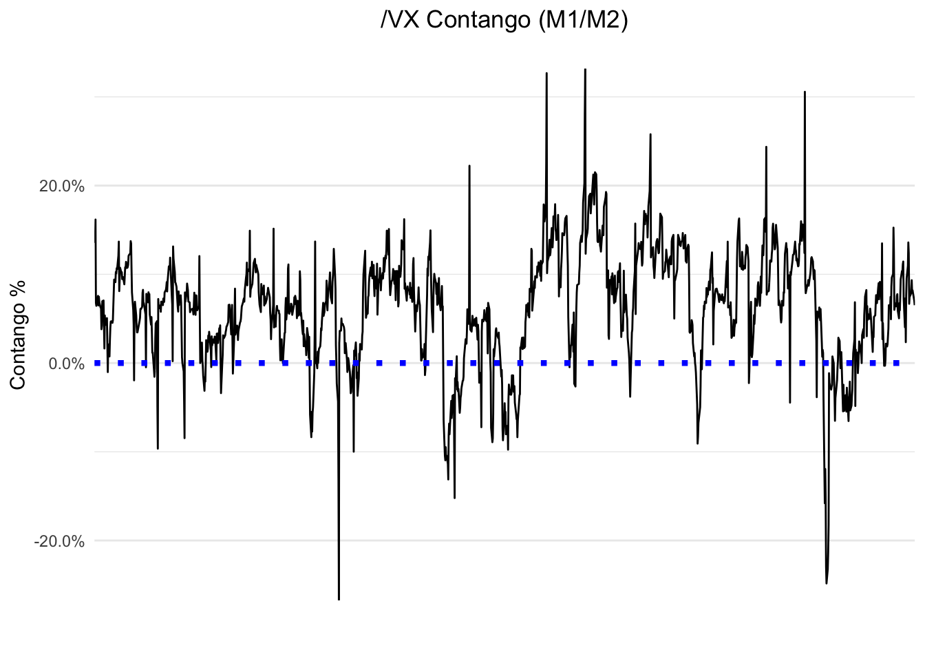
Volatility futures contracts are used in many trading strategies. The relationship between the prices of different maturities and the gap from the spot price can be tested as trade entry criteria. In this post we will connect to the CBOE site and download the historical /VX futures data so that we can then calculate contango to use in future analysis.
Download the data from CBOE site
url <- "https://markets.cboe.com/us/futures/market_statistics/historical_data/"
page <- xml2::read_html(url)
regex_vx <- "(VX){1}[+](VXT){1} " # RegEx for VX files on site

files <- page %>%
  html_nodes("a") %>%
  html_text() %>%
  str_squish()

paths <- page %>%
  html_nodes("a") %>%
  html_attr("href")

links <- data.frame(path = paths, file = files) %>%
  mutate(link = paste0(url, path),
         file_name = paste0(here::here(), "/static/data/vx_history/",
                            file, ".csv")) %>%
  filter(str_detect(file, regex_vx))

pwalk(list(url = links$link, destfile = links$file_name), download.file)
Data Processing
Bind files
Split contract name into year, month, contract symbol
Calculate contango as % of (front month - back month) / front month
Add front month and back month as new columns for reference
vx_files = as.data.frame(
  list.files(paste0(here::here(), "/static/data/vx_history"), pattern = ".csv"),
  stringsAsFactors = FALSE) %>%
  setNames("file_name") %>%
  mutate(file_name = paste0(here::here(), "/static/data/vx_history/", file_name))

vx_data <- map_df(vx_files$file_name, read.table,
                  blank.lines.skip = TRUE, fill = TRUE, header = TRUE,
                  quote = '', sep = ",", stringsAsFactors = FALSE) %>%
  setNames(c("quote_date", "contract", "open", "high", "low", "close",
             "settle", "change", "volume", "efp", "open_interest")) %>%
  mutate(quote_date = as.Date(quote_date, format = "%Y-%m-%d"),
         contract = gsub("\\(", "", contract),
         contract = gsub("\\)", "", contract)) %>%
  separate(contract, c("contract", "month", "year"), sep = " ") %>%
  mutate(month = as.yearmon(month, "%b"),
         month = month(month)) %>%
  mutate_at(vars(4:13), funs(as.numeric)) %>%
  group_by(quote_date) %>%
  arrange(year, month) %>%
  mutate(contango = c(NA, diff(settle)),
         diff_month = lead(contango, 1),
         diff_front_back = nth(diff_month, 1),
         contango_perc = diff_front_back / first(settle),
         front_month = nth(settle, 1),
         back_month = nth(settle, 2)) %>%
  select(quote_date, front_month, back_month,
         diff_front_back, contango_perc) %>%
  group_by(quote_date) %>%
  distinct() %>%
  ungroup() %>%
  filter(complete.cases(.)) %>%
  arrange(desc(quote_date))
Printing recent dates to show data most important variables and structure
for_vx_data <- vx_data %>%
  mutate(contango_perc = percent(contango_perc, accuracy = .01))

kable(head(for_vx_data), digits = 2, format = "html",
      caption = "/VX Contango",
      col.names = c("Date", "Front Month", "Back Month", "Diff", "Contango"),
      escape = FALSE,
      align = c("l", "r", "r", "r", "r")) %>%
  kable_styling(bootstrap_options = "striped", position = "center",
                full_width = FALSE) %>%
  column_spec(1:5, width = "1.25in")
| Date | Front Month | Back Month | Diff | Contango |
|---|---|---|---|---|
| 2018-09-05 | 14.57 | 15.53 | 0.95 | 6.52% |
| 2018-09-04 | 14.22 | 15.22 | 1.00 | 7.03% |
| 2018-08-31 | 14.03 | 15.18 | 1.15 | 8.20% |
| 2018-08-30 | 14.53 | 15.68 | 1.15 | 7.92% |
| 2018-08-29 | 13.93 | 15.22 | 1.30 | 9.34% |
| 2018-08-28 | 14.07 | 15.28 | 1.20 | 8.53% |
Historical Contango
ggplot(data = vx_data, aes(x = quote_date, y = contango_perc)) +
  geom_line() +
  geom_hline(yintercept = 0, linetype = "dotted", color = "blue", size = 1.5) +
  theme_minimal() +
  theme(plot.title = element_text(hjust = 0.5)) +
  scale_x_discrete(labels = "Date") +
  scale_y_continuous(labels = scales::percent) +
  xlab("") +
  ylab("Contango %") +
  ggtitle("/VX Contango (M1/M2)")

We can now use this data in future posts on trading strategy analysis.
If you have suggestions for studies, improvements for rstats code, or any other feedback please reach out with the contact links on the sidebar
